1. Running a pre-defined set

This tutorial will describe how to run the model with a default set of parameters and create some simple plots from the output data.

1.1 First run

To run the program, open the command prompt and change the directory cd to that of the executable file gdsimsapp. Then, run the application. This step will look different depending on your operating system. For example, on Windows:

cd C:\Users\MyUser\Projects\GeneralMetapop\build
gdsimsapp.exe

This will display the command-line interface:

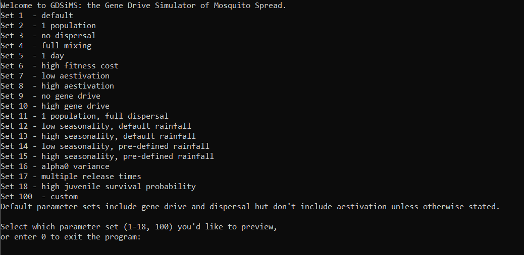
The interface provides default sets of parameters to demonstrate specific behaviours. Let’s try running set 1.

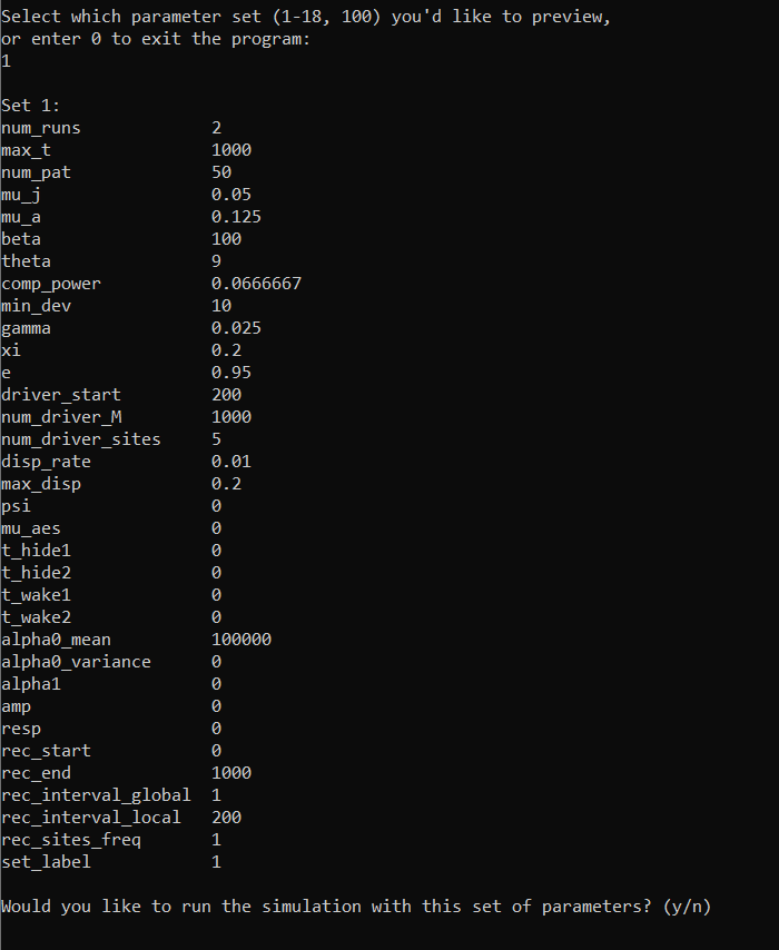
Upon entering 1, the program will give us a preview of the set 1 parameters (the full explanation of parameters can be found in the InputParams documentation - we will introduce some of these in the following tutorials). Since we’re happy with these parameters, we can enter y to run the program.

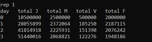
This will run the simulation, displaying some data to show how the simulation is progressing:

Note

The data will take a while to start showing on screen at the start of each run. This is because the simulation implicitly runs what is known in computational modelling as a ‘burn-in period’. This is a period of time given to the populations being modelled so they can reach a stable equilibrium, before any interventions can be applied to them. In our model, the burn-in period is 1 year (365 days). We discard this data and start recording from here.

On the first column we have the simulation day. This will run up to 1000 days, since we have chosen max_t = 1000. The following four columns display the total number of juvenile mosquitoes (J), adult male mosquitoes (M), adult virgin (unmated) females (V) and adult (mated) females (F).

Since this set includes two repetitions (num_runs = 2), the days will restart upon the second repetition.

At the end of the simulation we’ll be able to see the program runtime.

Looking at the output data

The program run will have created a new subdirectory in our build directory called output_files. This contains all the output files generated by the program. There are text files of three types:

• CoordinateList.txt: contains the (x, y) coordinates of all the patches in the simulation (in our set 1 we used num_pat = 50).

• Totals.txt: contains the total adult mated female mosquito numbers across all patches as simulation time passes. These are divided into the different genotypes available (more information on genotypes in Tutorial 3.2 Model introduction: Gene drive).

• LocalData.txt: contains the adult mated female mosquito numbers, divided by genotype, at each patch over time.

The program will generate a set of these files for each repetition (also called run).

1.2 Simple plots: coordinates and totals (optional - python)

The output files we have obtained can be plotted in various ways. Let’s look at how to make some simple plots on Python. Feel free to skip this vignette if you’d like to use a different language.

The test directory you cloned from GitHub will contain a plotting script called GeneralMetapopPlots.py with the code for these examples.

Required installations for this tutorial

• python (and a suitable IDE)

• numpy package

• matplotlib package

Plotting the coordinates

The following code will plot the patch coordinates for run 1 of the set we just ran. Make sure to have your directory set to output_files.

test/GeneralMetapopPlots.py - ‘Plot coordinates of patches’

import numpy as np
import matplotlib.pyplot as plt

# extract data from the file
coords = np.loadtxt("CoordinateList1run1.txt", skiprows=2)

x = coords[:, 1] # second column
y = coords[:, 2] # third column

plt.figure()
plt.title("Patch locations")
plt.xlabel("x (km)")
plt.ylabel("y (km)")
plt.scatter(x, y, marker='.')

Notice how we skip the first two rows of the table containing the header labels. We also ignore the first column since it only contains the patch index numbers.

This script will generate the following plot:

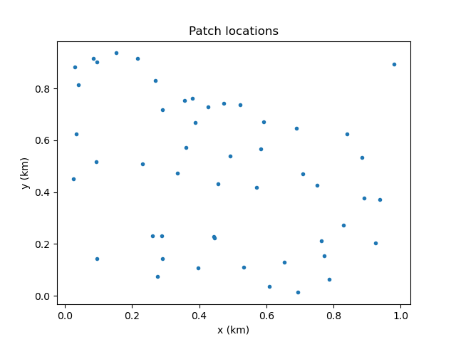
Now we can see the spatial distribution of the patches!

Note

Plots may look slightly different on different systems due to differences in random number generation in the model between systems. Output data for these tutorials has been generated on a Windows 10 with g++ compiler v13.1.0.

Plotting total females over time

The following code will plot the total adult mated female mosquito numbers for the first run of set 1. We can plot several lines corresponding to the different genotypes so we can observe the changes in genotypic composition over time.

test/GeneralMetapopPlots.py - ‘Plot global output (totals) from model’

import numpy as np
import matplotlib.pyplot as plt

# extract data from the file
totals = np.loadtxt("Totals1run1.txt", skiprows=2)
times = totals[:, 0]
total_females = totals[:, 1:]

plt.figure()
plt.title("Total mated females across the area")
plt.xlabel("Day")
plt.ylabel("Total number of individuals")
plt.plot(times, total_females[:, 0], label="$F_{WW}$")
plt.plot(times, total_females[:, 1], label="$F_{WD}$")
plt.plot(times, total_females[:, 2], label="$F_{DD}$")
plt.plot(times, total_females[:, 3], label="$F_{WR}$")
plt.plot(times, total_females[:, 4], label="$F_{RR}$")
plt.plot(times, total_females[:, 5], label="$F_{DR}$")

As before, make sure to skip the first two rows of the table.

This script will generate the following plot:

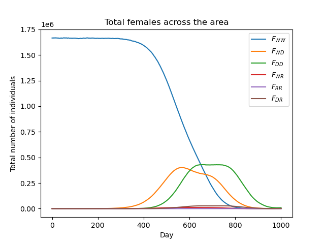
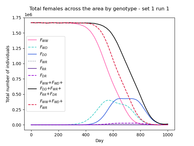
We can now clearly see how the composition of the overall mosquito population evolves over time!