Usage

The GUI provides features to enter model parameters, run the model program and view the output data.

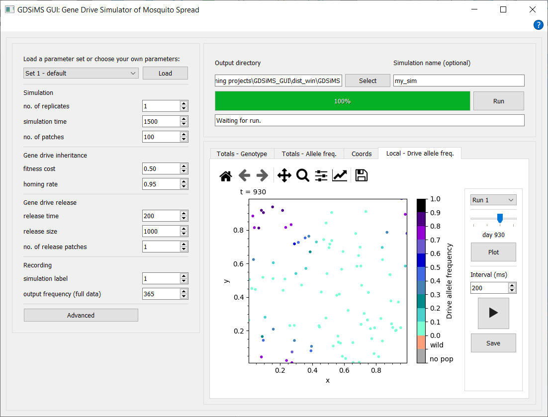
1. Load a parameter set from available pre-defined sets by selecting one from the drop-down and clicking Load. Parameters can also be tweaked at any time before running, including those in the advanced parameter window dialog. All parameter labels have tooltips which display descriptions when you hover over them.

2. Select an output data destination directory (i.e. folder) and choose the name for your simulation before clicking Run. The interface will give updates on the simulation’s progress whilst it’s running, and plotting options will become available upon completion of the simulation.

   Note

   The GUI won’t allow simulation folder names (in the same output destination folder) that have already been used to run a simulation. This is to prevent over-writing of files and confusion.

3. Choose from the tabs to view different plot and animation options, interact via the plot sidebar to select plotting parameters and click Plot or Play to update the canvas.

Caution

If the simulation has issues when running, please attempt to click the Abort button (which replaces the Run button when the simulation is running) before closing the window. Aborting may take a while and may freeze the application as it’s an intensive and last-resort process but if 1-2 mins have passed with no change, force quit the application.

Output files

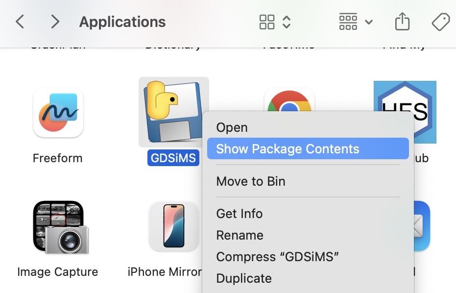
By default, the output files will be created in the _internal subfolder for Windows (found in the folder you ran the GDSiMS.exe file from), and in the app’s Contents/Frameworks/ subfolder for Mac. You can access the app’s contents on Mac by right-clicking on the GDSiMS app in your Applications folder and choosing “Show Package Contents”.

Alternatively, an output destination directory (i.e. folder) can be selected on the GUI before running the simulation.

A simulation folder will be created at the output destination upon each simulation run. The name of this folder will be the simulation name you provided before running. This is optional and if not provided, the app will name the folder with a date-time stamp of the simulation start time.

Three objects are created in the simulation folder:

• params.txt file - file fed into the model program.

• paramsInfo.csv file - contains all parameter values used in the simulation and parameter descriptions.

• output_files folder - contains data files produced by the model program. More detail on these in the model program’s Output files documentation page.

Pre-defined parameter sets

The values for the pre-defined parameter sets in the GDSiMS GUI are below. These sets are different to the ones provided by GDSiMS. More information on model parameters can be found in the model program’s User Guide

		Set 1	Set 2	Set 3	Set 4	Set 5	Set 6
Parameter	Model program equivalent	default	low fitness cost	high fitness cost	high number of release sites	low dispersal rate	high dispersal rate
no. of replicates	num_runs	1	1	1	1	1	1
simulation time	max_t	1500	1500	1500	1500	1500	1500
no. of patches	num_pat	100	100	100	100	100	100
juvenile mortality rate	mu_j	0.05	0.05	0.05	0.05	0.05	0.05
adult mortality rate	mu_a	0.125	0.125	0.125	0.125	0.125	0.125
mating rate factor	beta	100.0	100.0	100.0	100.0	100.0	100.0
egg laying rate	theta	9.0	9.0	9.0	9.0	9.0	9.0
juvenile survival factor	comp_power	0.066666667	0.066666667	0.066666667	0.066666667	0.066666667	0.066666667
juvenile min. development time	min_dev	10	10	10	10	10	10
resistance formation rate	gamma	0.025	0.025	0.025	0.025	0.025	0.025
fitness cost	xi	0.5	0.5	0.5	0.5	0.5	0.5
homing rate	e	0.95	0.95	0.95	0.95	0.95	0.95
release time	driver_start	200	200	200	200	200	200
release size	num_driver_M	1000	1000	1000	1000	1000	1000
no. of release patches	num_driver_sites	1	1	1	1	1	1
dispersal rate	disp_rate	0.01	0.01	0.01	0.01	0.01	0.01
max. dispersal distance	max_disp	0.2	0.2	0.2	0.2	0.2	0.2
aestivation rate	psi	0.0	0.0	0.0	0.0	0.0	0.0
aestivation mortality	mu_aes	0.0	0.0	0.0	0.0	0.0	0.0
start hiding date	t_hide1	0	0	0	0	0	0
end hiding date	t_hide2	0	0	0	0	0	0
start waking date	t_wake1	0	0	0	0	0	0
end waking date	t_wake2	0	0	0	0	0	0
population size factor	alpha0_mean	100000.0	100000.0	100000.0	100000.0	100000.0	100000.0
population size variance	alpha0_variance	0.0	0.0	0.0	0.0	0.0	0.0
rainfall contribution to pop. size	alpha1	0.0	0.0	0.0	0.0	0.0	0.0
rainfall seasonality	amp	0.0	0.0	0.0	0.0	0.0	0.0
responsiveness to rainfall	resp	0.0	0.0	0.0	0.0	0.0	0.0
output start (full data)	rec_start	200	200	200	200	200	200
output end (full data)	rec_end	1500	1500	1500	1500	1500	1500
output frequency (summary data)	rec_interval_global	1	1	1	1	1	1
output frequency (full data)	rec_interval_local	365	365	365	365	365	365
local site freq.	rec_sites_freq	1	1	1	1	1	1
simulation label	set_label	1	2	3	4	5	6
dispersal type		Radial	Radial	Radial	Radial	Radial	Radial
boundary type		Toroid	Toroid	Toroid	Toroid	Toroid	Toroid
rainfall file		None	None	None	None	None	None
patch coordinates file		None	None	None	None	None	None
release times file		None	None	None	None	None	None

Advanced parameter window

Advanced parameters can be accessed by clicking the Advanced button at the bottom of the parameters section. For more information on the model’s advanced options visit the Advanced options page.

Note that patch coordinates file selection will only show when an Edge boundary type is selected.

Also note that the default dispersal type in the GUI is Radial - this differs from GDSiMS, where the default is Distance kernel.

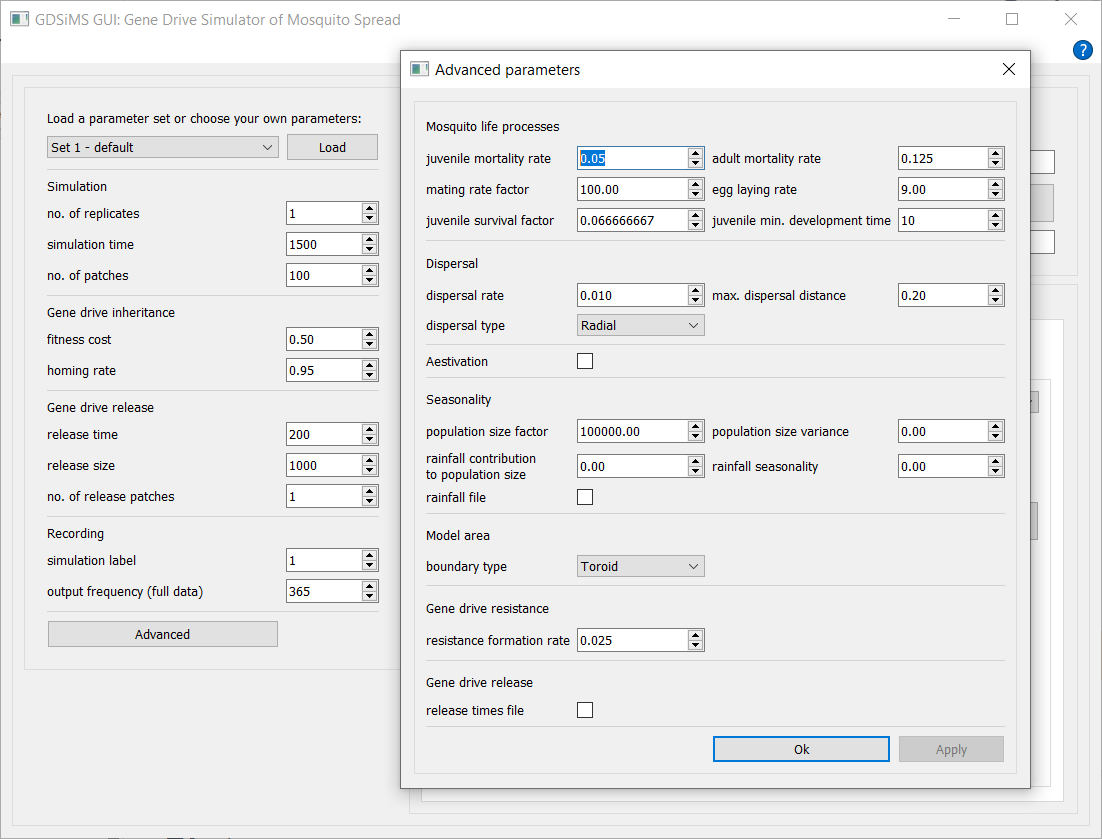
Caution

If the advanced parameter window is closed with the close button, changes won’t be applied. Please use the Ok or Apply buttons to confirm changes.

Plots

Each plot tab has a navigation bar above the plot canvas which can be used to save the figure, modify axes labels, titles, change the type of axes scales…

Each tab also has an interaction section where run number (i.e. simulation repetition index) can be selected from the drop-down and plotted. Other options are provided depending on the plot.

Current plot tabs available:

Totals - Genotype

A plot of the total number of adult male mosquitoes over all sites for each day of the simulation. This includes plot lines for the different genotypes modelled - plot lines can be selected and re-plotted by clicking Plot again. Hover over the labels in the interaction sidebar to see descriptions for these. This plot uses data from the Totals file. W is a wild-type allele, D is a drive-type allele and R is a non-functional resistance allele.

Totals - Allele frequency

Similar to the above, where allele frequencies for the wild-type (W), drive-type (D) and non-functional resistance alleles (R) over the six available genotype combinations and over time have been calculated.

e.g. for wild-type allele on one day

\[\text{W}_{\text{freq}} = \frac{\text{M}_{\text{WW}} + \text{M}_{\text{WD}} + \text{M}_{\text{WR}}}{\text{M}_{\text{WW}} + \text{M}_{\text{WD}} + \text{M}_{\text{DD}} + \text{M}_{\text{WR}} + \text{M}_{\text{RR}} + \text{M}_{\text{DR}}}\]

Coordinates

Patch coordinates plot of all modelled population sites using data from the Coordinates output file.

Local - drive allele frequency

This combines a plot and an animation option in the same plotspace. Adjust the slider and click Plot to (re-)plot a snapshot of the local populations’ (i.e. patches’) drive allele frequencies at the chosen simulation day. Alternatively, choose the frame interval for the animation and click the Play button. This animation can be saved as a GIF file by clicking Save. The plot and animation use data from the Coordinates output file and Local data file.

Note

Plots will not be plotted (or updated) until the Plot button of the respective tab is clicked.